Clustering analysis in R, with factoextra and NbClust
I recently gave a small talk on some packages I like using for doing clustering analysis in R. Here’s a brief introduction to some features of factoextra and NbClust
There are many libraries and functions in R for performing clustering analysis, so why look at these 2? Well, they solve two important challenges with clustering: visualisation and determining the optimal number of clusters.
In general, cluster analysis is an unsupervised machine learning task, meaning we don’t predefine a target output for the learning. For clustering, this mainly means that we don’t know what the categories will be before we start the analysis. We also don’t know how many clusters are present.
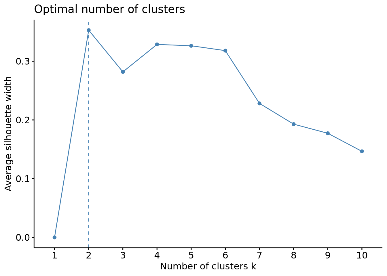
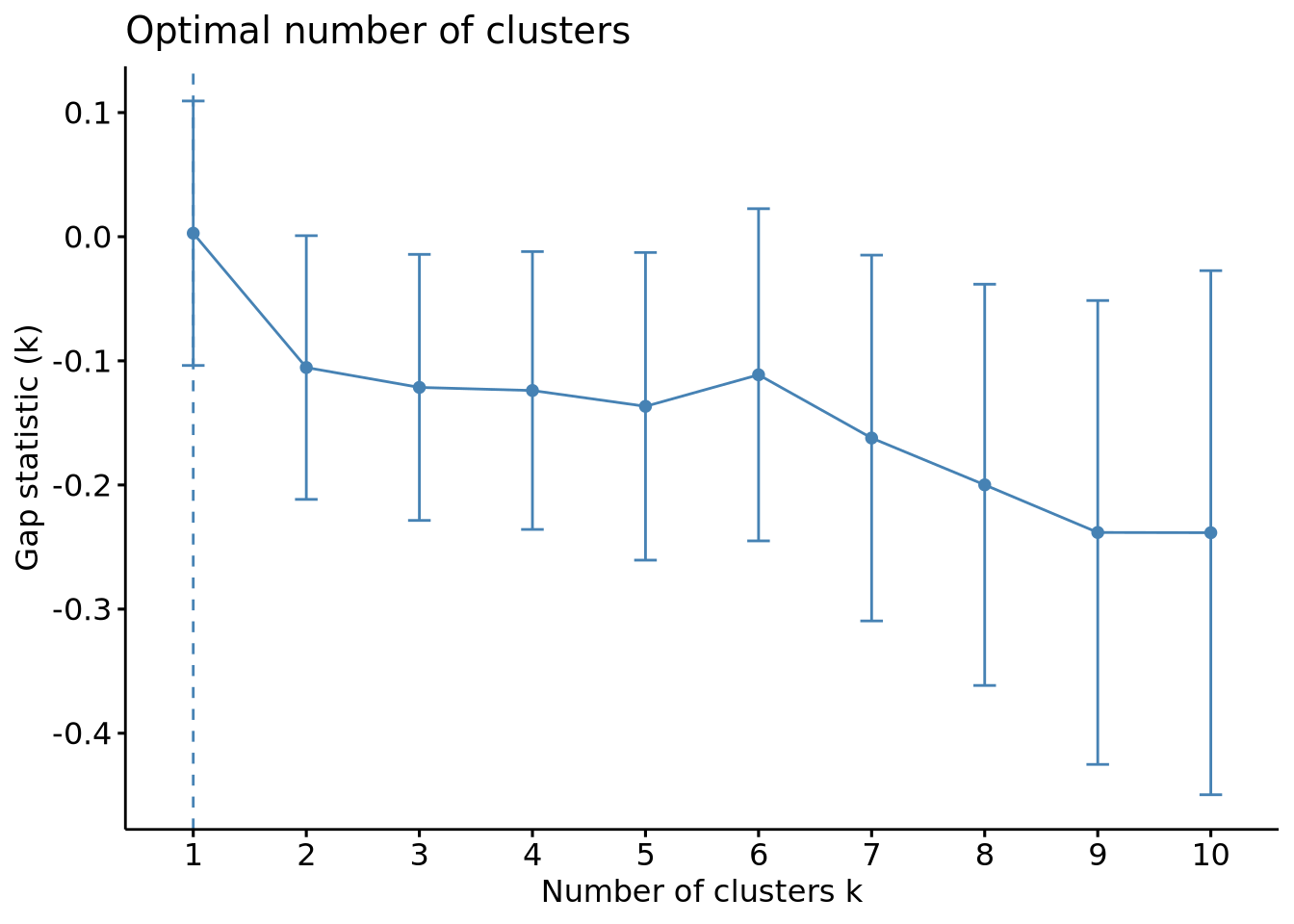
Many indices have been created to help with determining the optimal number of clusters, however these each have their own advantages and disadvantages and often give conflicting results. We’ll demonstrate this by looking at the results from three popular graphical methods: elbow plot, silhouette, and gap statistic.
Dataset
We’ll be looking at data from the Soundscape Indices (SSID) Database. This dataset contains data in-situ perceptual assessments of urban soundscapes, paired with acoustic and environmental data. For this set, we’ll be looking at the perceptual data only.
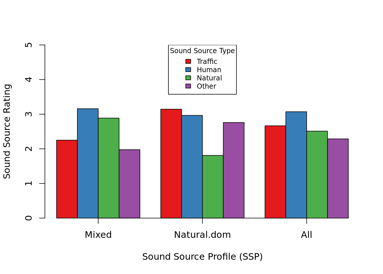
To collect the data, random members of the public were approached while in urban public spaces and asked to take a survey about how they perceive the sound environment. A section of the questions ask specifically about the perceived dominance of sound sources in the space. Sound sources are categorized as Traffic noise, Other noise, Human sounds, Natural sounds, and are rated from 1 [not at all] to 5 [dominates completely].
The data was collected across 27 locations in the UK, Italy, Spain, the Netherlands, and China. The goal here is to investigate whether these locations can be categorized based on their composition of sound sources.
Code
library(readxl)library(dplyr) # Data processing and piping# Clustering librarieslibrary(factoextra) # Clustering and visualisationlibrary(NbClust) # Optimal Number of Clusterslibrary(RCurl) # For downloading data from Zenodotemp.file <-paste0(tempfile(), ".xlsx")download.file("https://zenodo.org/record/5705908/files/SSID%20Lockdown%20Database%20VL0.2.2.xlsx", temp.file, mode="wb")ssid.data <-read_excel(temp.file)vars <-c("Traffic", "Other", "Natural", "Human")# vars <- c("pleasant", "chaotic", "vibrant", "uneventful", "calm", "annoying", "eventful", "monotonous")# Cutdown the datasetssid.data <- ssid.data[c("GroupID", "SessionID", "LocationID", vars)]# ssid.data <- subset(ssid.data, Lockdown != 1)# Set GroupID, SessionID, Location as factor typessid.data <- ssid.data %>%mutate_at(vars(GroupID, SessionID, LocationID),funs(as.factor))ssid.data <- ssid.data %>%mutate_at(vars(vars),funs(as.numeric))# Calculate the mean response for each GroupIDssid.data <- ssid.data %>%group_by(GroupID) %>%summarize(Traffic =mean(Traffic, na.rm=TRUE),Other =mean(Other, na.rm=TRUE),Natural =mean(Natural, na.rm=TRUE),Human =mean(Human, na.rm=TRUE),# pleasant = mean(pleasant, na.rm = TRUE),# chaotic = mean(chaotic, na.rm = TRUE),# vibrant = mean(vibrant, na.rm = TRUE),# uneventful = mean(uneventful, na.rm = TRUE),# calm = mean(calm, na.rm = TRUE),# annoying = mean(annoying, na.rm = TRUE),# eventful = mean(eventful, na.rm = TRUE),# monotonous = mean(monotonous, na.rm = TRUE),LocationID = LocationID[1])# analysis.data$LocationID <- unique(ssid.data[c('GroupID', 'LocationID')])['LocationID']ssid.data <-na.omit(ssid.data)knitr::kable(head(ssid.data))
Note: If the data use different scales, they should always be standardised before clustering. In this case, all of the data are on the same scale, so we don’t need to worry.
As we can see, it can be less than obvious how to interpret some of these - where exactly is the ‘elbow’ in the elbow plot? Silhouette pretty clearly says k = 2, but the Gap stat gives k = 1, which isn’t very useful. How do we know which is right?
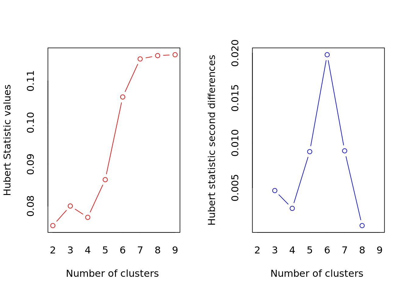
*** : The Hubert index is a graphical method of determining the number of clusters.
                In the plot of Hubert index, we seek a significant knee that corresponds to a
                significant increase of the value of the measure i.e the significant peak in Hubert
                index second differences plot.
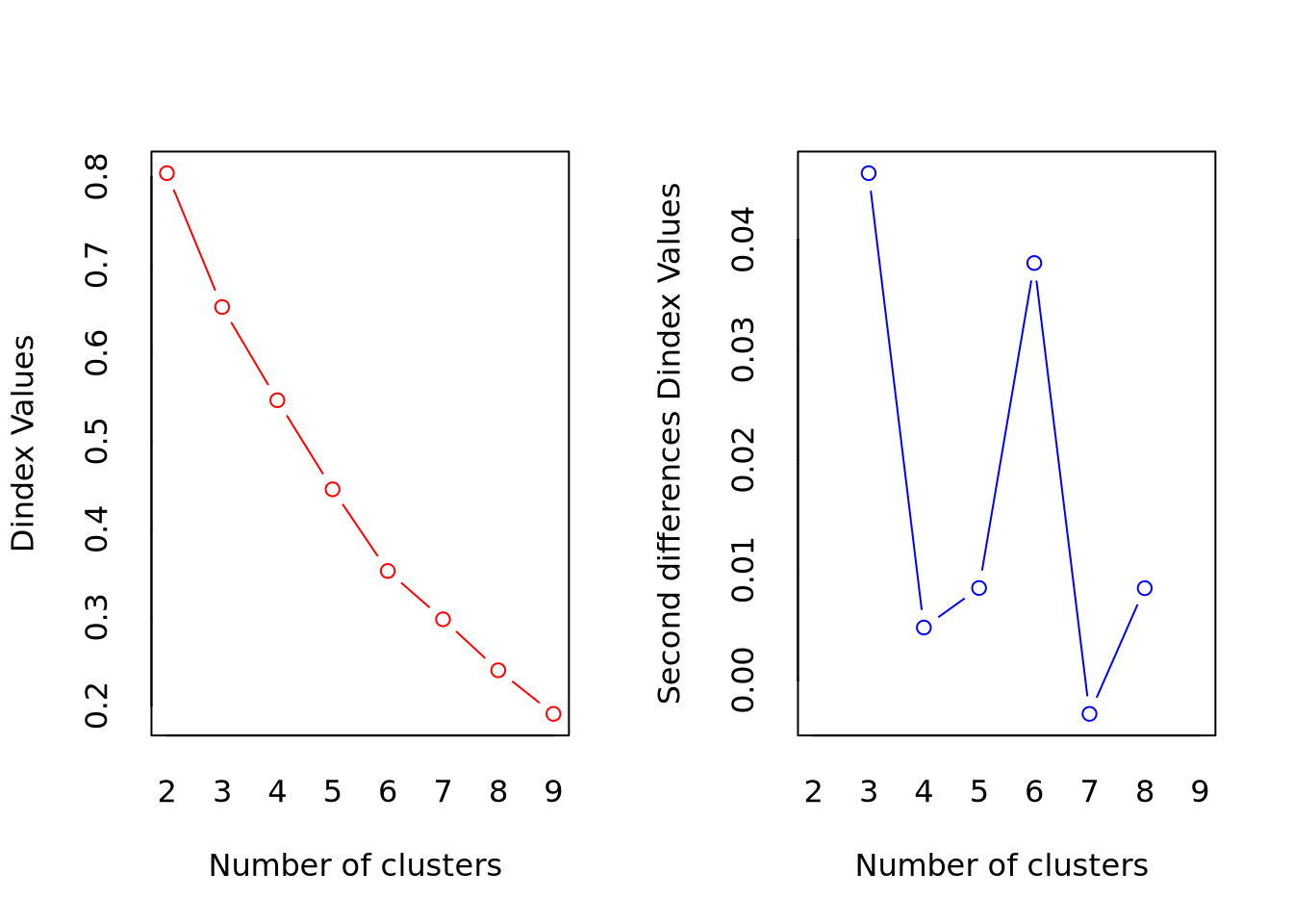
*** : The D index is a graphical method of determining the number of clusters.
                In the plot of D index, we seek a significant knee (the significant peak in Dindex
                second differences plot) that corresponds to a significant increase of the value of
                the measure.

*******************************************************************
* Among all indices:
* 9 proposed 2 as the best number of clusters
* 4 proposed 3 as the best number of clusters
* 2 proposed 4 as the best number of clusters
* 1 proposed 5 as the best number of clusters
* 4 proposed 6 as the best number of clusters
* 1 proposed 7 as the best number of clusters
* 2 proposed 8 as the best number of clusters
* 5 proposed 9 as the best number of clusters

                   ***** Conclusion *****

* According to the majority rule, the best number of clusters is  2


*******************************************************************
Code
knitr::kable(res)
KL
CH
Hartigan
CCC
Scott
Marriot
TrCovW
TraceW
Friedman
Rubin
Cindex
DB
Silhouette
Duda
Pseudot2
Beale
Ratkowsky
Ball
Ptbiserial
Gap
Frey
McClain
Gamma
Gplus
Tau
Dunn
Hubert
SDindex
Dindex
SDbw
2
1.0970
8.1449
6.0597
7.5851
102.6537
30.2615
13.4952
10.1742
351.3546
36.9377
0.4269
0.8174
0.3529
0.6156
4.9946
1.3398
0.3840
5.0871
0.5020
-0.9326
1.0370
0.4096
0.5903
3.7821
10.8974
0.3539
0.0753
2.5622
0.8042
0.4459
3
1.1005
8.4961
5.2330
6.3990
119.6026
18.4865
5.5195
6.5603
404.1006
57.2860
0.3951
1.0948
0.2818
0.4299
5.3038
2.5609
0.4103
2.1868
0.4710
-1.6230
0.2765
1.3913
0.6265
3.1026
10.4103
0.3626
0.0800
2.8643
0.6523
0.3387
4
1.6303
9.3352
3.5123
5.9285
136.6838
8.8328
2.0114
4.3066
514.5025
87.2635
0.5492
0.8335
0.3286
2.5977
-1.2301
-0.9899
0.4303
1.0767
0.4840
-1.8404
0.2171
2.0924
0.7560
1.5513
9.6154
0.5689
0.0773
2.4025
0.5465
0.2559
5
0.8819
9.4327
4.1056
5.4008
150.1412
4.9017
0.9988
3.0977
615.3276
121.3182
0.5171
0.6492
0.4032
2.6324
-1.2402
-0.9981
0.4026
0.6195
0.4854
-2.3510
0.1834
2.4726
0.8391
0.8718
9.0897
0.6139
0.0863
2.3482
0.4455
0.1689
6
2.4474
10.7100
1.9565
5.2900
170.5431
1.4694
0.3679
2.0471
969.8285
183.5792
0.5973
0.5852
0.4719
1.8668
-0.4643
-0.5605
0.3812
0.3412
0.4830
-2.4797
0.5241
2.9403
0.9529
0.2051
8.3077
0.8559
0.1062
2.4432
0.3528
0.1185
7
0.9458
10.0676
1.9696
4.5460
183.1309
0.7595
0.2213
1.5999
1194.4928
234.8889
0.5305
0.5508
0.4589
3.4939
-0.7138
-0.8616
0.3578
0.2286
0.4476
-2.9193
0.8670
3.6092
0.9643
0.1282
6.9231
0.8905
0.1153
3.0849
0.2980
0.0970
8
0.9554
9.7863
2.1072
4.5678
213.5276
0.0957
0.1542
1.2045
3652.8265
311.9964
0.4860
0.4826
0.5005
3.0804
-0.6754
-0.8152
0.3386
0.1506
0.3947
-3.0908
0.5258
4.8153
0.9537
0.1282
5.2821
0.7320
0.1161
3.2357
0.2402
0.0697
9
0.9437
9.9481
2.5926
3.7773
235.4352
0.0225
0.0873
0.8474
6052.3637
443.4830
0.4147
0.4100
0.5619
4.7507
0.0000
0.0000
0.3219
0.0942
0.3339
-3.4867
0.1666
7.0102
0.9662
0.0641
3.6667
0.7386
0.1163
3.4232
0.1907
0.0490
CritValue_Duda
CritValue_PseudoT2
Fvalue_Beale
CritValue_Gap
2
0.2019
31.6230
0.2766
0.7534
3
0.0160
246.4030
0.0787
0.2949
4
-0.1694
-13.8056
1.0000
0.6048
5
-0.1694
-13.8056
1.0000
0.2346
6
-0.3257
-4.0703
1.0000
0.5672
7
-0.3257
-4.0703
1.0000
0.3163
8
-0.3257
-4.0703
1.0000
0.5663
9
-0.5879
0.0000
NaN
0.3864
KL
CH
Hartigan
CCC
Scott
Marriot
TrCovW
TraceW
Friedman
Rubin
Cindex
DB
Silhouette
Duda
PseudoT2
Beale
Ratkowsky
Ball
PtBiserial
Gap
Frey
McClain
Gamma
Gplus
Tau
Dunn
Hubert
SDindex
Dindex
SDbw
Number_clusters
6.0000
6.00
6.0000
2.0000
8.0000
4.0000
3.0000
3.0000
8.000
6.0000
3.0000
9.00
9.0000
2.0000
2.0000
2.0000
4.0000
3.0000
2.000
2.0000
2.000
2.0000
9.0000
9.0000
2.0000
7.0000
0
5.0000
0
9.000
Value_Index
2.4474
10.71
2.1492
7.5851
30.3968
5.7226
7.9756
1.3603
2458.334
-10.9512
0.3951
0.41
0.5619
0.6156
4.9946
1.3398
0.4303
2.9003
0.502
-0.9326
1.037
0.4096
0.9662
0.0641
10.8974
0.8905
0
2.3482
0
0.049
x
CamdenTown
1
EustonTap
1
MarchmontGarden
2
MonumentoGaribaldi
2
PancrasLock
2
RegentsParkFields
2
RegentsParkJapan
2
RussellSq
2
SanMarco
2
StPaulsCross
2
StPaulsRow
2
TateModern
2
TorringtonSq
1
Code
fviz_nbclust(res)
Error in if (class(best_nc) == "numeric") print(best_nc) else if (class(best_nc) == : the condition has length > 1
Code
k =2k.fit <-kmeans(means, k)knitr::kable(k.fit)
Error in as.data.frame.default(x): cannot coerce class '"kmeans"' to a data.frame
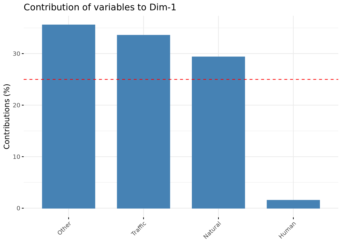
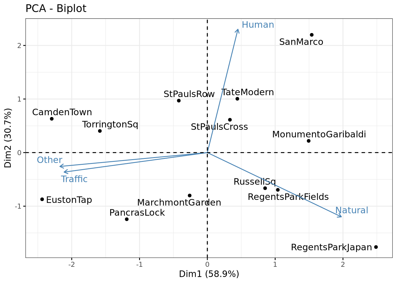
           name      Dim.1      Dim.2     coord      cos2  contrib
Traffic Traffic -0.8891690 -0.1531570 0.8140785 0.8140785 22.70701
Other     Other -0.9153206 -0.1088317 0.8496561 0.8496561 23.69937
Natural Natural  0.8316428 -0.5046107 0.9462617 0.9462617 26.39398
Human     Human  0.1897201  0.9690987 0.9751460 0.9751460 27.19965
Code
fviz_contrib(res.pca, "var")
Code
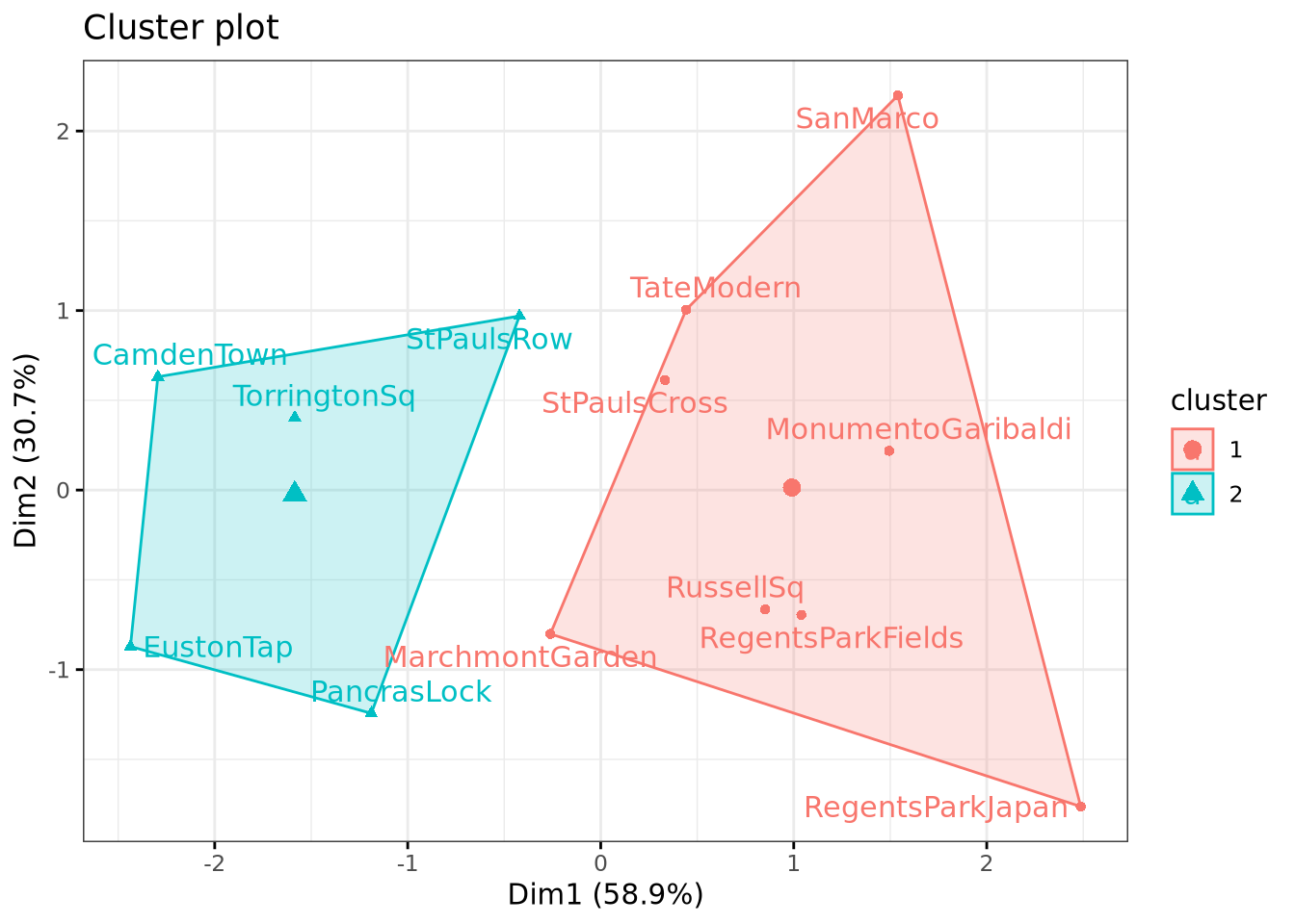
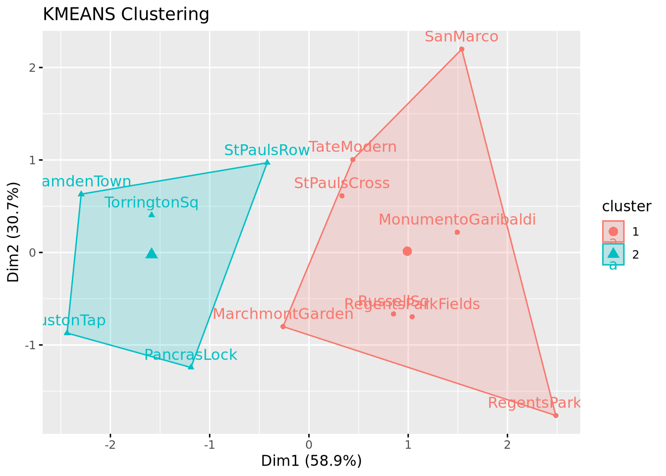
fit <-eclust(means, "kmeans", k=k)
Code
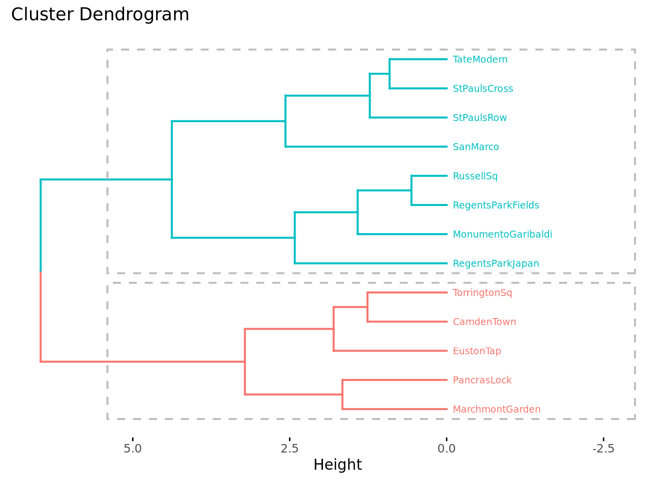
h.fit <-eclust(means, "hclust", k=k, stand = T, hc_method ="ward.D2")
Warning: The `<scale>` argument of `guides()` cannot be `FALSE`. Use "none" instead as
of ggplot2 3.3.4.
ℹ The deprecated feature was likely used in the factoextra package.
  Please report the issue at <https://github.com/kassambara/factoextra/issues>.
Code
fviz_dend(h.fit, labels_track_height =2.5, horiz=TRUE, rect =TRUE, cex =0.5)
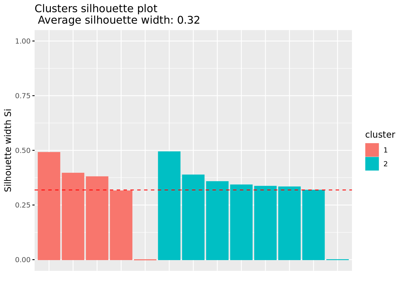
Silhouette (Si) analysis is a cluster validation approach that measures how well an observation is clustered and it estimates the average distance between clusters.
Details
Observations with a large silhouette Si (almost 1) are very well clustered
A small Si (around 0) means that the observation lies between two clusters
Observations with a negative Si are probably placed in the wrong cluster
Code
fviz_silhouette(h.fit)
  cluster size ave.sil.width
1       1    5          0.32
2       2    8          0.32
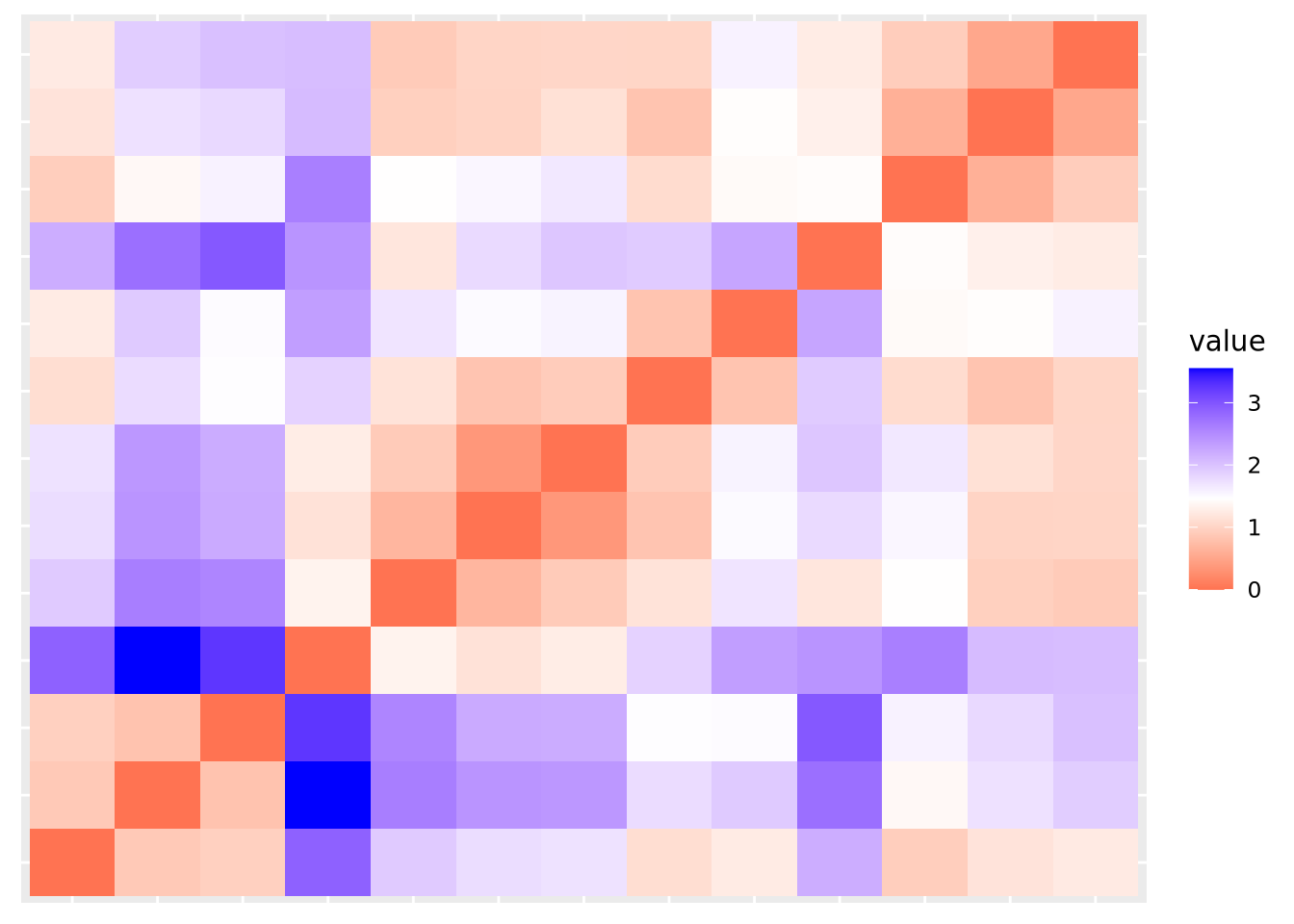
get_clust_tendency
Before applying cluster methods, the first step is to assess whether the data is clusterable, a process defined as the assessing of clustering tendency. get_clust_tendency() assesses clustering tendency using Hopkins’ statistic and a visual approach.
Details
Hopkins Statistic: If the value of Hopkins statistic is close to 1 (far above 0.5), then we can conclude that the dataset is significantly clusterable.
@online{mitchell2020,
  author = {Mitchell, Andrew},
  title = {Clustering Analysis in {R,} with `Factoextra` and
    {`NbClust`}},
  date = {2020-06-18},
  url = {https://drandrewmitchell.com/posts/2020-06-18_cluster-analysis-in-r/},
  langid = {en}
}