Introduction to SSM Analysis
This notebook provides an introduction to Structural Summary Method (SSM) analysis using the circumplex package.
1. Loading Example Data: jz2017
We’ll use the jz2017 dataset from Zimmermann & Wright (2017). This
dataset includes self-report data from 1166 undergraduate students who
completed:
- A circumplex measure of interpersonal problems (IIP-SC) with eight subscales: PA, BC, DE, FG, HI, JK, LM, NO
- A measure of personality disorder symptoms with ten subscales: PARPD, SCZPD, SZTPD, ASPD, BORPD, HISPD, NARPD, AVPD, DPNPD, OCPD
| Gender | PA | BC | DE | FG | HI | JK | LM | NO | PARPD | SCZPD | SZTPD | ASPD | BORPD | HISPD | NARPD | AVPD | DPNPD | OCPD |
|---|---|---|---|---|---|---|---|---|---|---|---|---|---|---|---|---|---|---|
| Female | 1.5 | 1.5 | 1.25 | 1.0 | 2.0 | 2.5 | 2.25 | 2.5 | 4 | 3 | 7 | 7 | 8 | 4 | 6 | 3 | 4 | 6 |
| Female | 0.0 | 0.25 | 0.0 | 0.25 | 1.25 | 1.75 | 2.25 | 2.25 | 1 | 0 | 2 | 0 | 1 | 2 | 3 | 0 | 1 | 0 |
| Female | 0.0 | 0.0 | 0.0 | 0.0 | 0.0 | 0.0 | 0.0 | 0.0 | 0 | 1 | 0 | 4 | 1 | 5 | 4 | 0 | 0 | 1 |
| Male | 2.0 | 1.75 | 1.75 | 2.5 | 2.0 | 1.75 | 2.0 | 2.5 | 1 | 0 | 0 | 0 | 1 | 0 | 0 | 0 | 0 | 0 |
| Female | 0.25 | 0.5 | 0.25 | 0.0 | 0.0 | 0.0 | 0.0 | 0.0 | 0 | 0 | 0 | 0 | 1 | 0 | 0 | 1 | 0 | 0 |
2. Mean-Based SSM Analysis
Single Group Analysis
Let’s analyze the interpersonal problems of the average individual in
the dataset using ssm_analyze(). The function returns an SSM object
with results, scores, and analysis details.
# Define circumplex scales and their angular positions
scales = ["PA", "BC", "DE", "FG", "HI", "JK", "LM", "NO"]
angles = [90, 135, 180, 225, 270, 315, 360, 45]

# Run SSM analysis
results = ssm_analyze(data=jz2017, scales=scales, angles=angles)

# Display summary
results.summary()
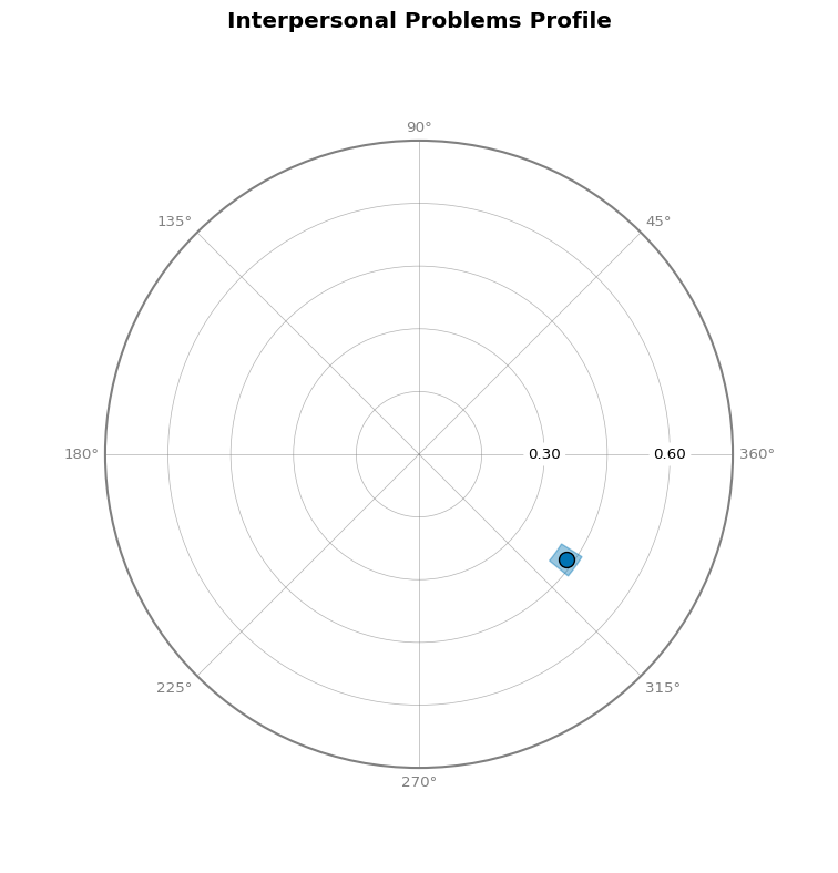
Statistical Basis:   Mean Scores
Bootstrap Resamples: 2000
Confidence Level:    0.95
Listwise Deletion:   True
Scale Displacements: [90.0, 135.0, 180.0, 225.0, 270.0, 315.0, 360.0, 45.0]


                  Profile[All]
┏━━━━━━━━━━━━━━┳━━━━━━━━━━┳━━━━━━━━━━┳━━━━━━━━━━┓
┃              ┃ Estimate ┃ Lower CI ┃ Upper CI ┃
┡━━━━━━━━━━━━━━╇━━━━━━━━━━╇━━━━━━━━━━╇━━━━━━━━━━┩
│ Elevation    │ 0.917    │ 0.889    │ 0.945    │
│ X-Value      │ 0.351    │ 0.323    │ 0.378    │
│ Y-Value      │ -0.252   │ -0.281   │ -0.223   │
│ Amplitude    │ 0.432    │ 0.402    │ 0.46     │
│ Displacement │ 324.292  │ 320.757  │ 327.79   │
│ Model Fit    │ 0.878    │          │          │
└──────────────┴──────────┴──────────┴──────────┘
Accessing Results
The SSM object provides easy access to results, scores, and analysis details:
# View results DataFrame with parameter estimates and confidence intervals
GT(results.results.round(2))
| Label | Group | Measure | e_est | e_lci | e_uci | x_est | x_lci | x_uci | y_est | y_lci | y_uci | a_est | a_lci | a_uci | d_est | d_lci | d_uci | fit_est |
|---|---|---|---|---|---|---|---|---|---|---|---|---|---|---|---|---|---|---|
| All | All | 0.92 | 0.89 | 0.95 | 0.35 | 0.32 | 0.38 | -0.25 | -0.28 | -0.22 | 0.43 | 0.4 | 0.46 | 324.29 | 320.76 | 327.79 | 0.88 |
| Label | PA | BC | DE | FG | HI | JK | LM | NO |
|---|---|---|---|---|---|---|---|---|
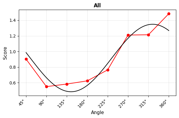
| All | 0.55 | 0.58 | 0.62 | 0.76 | 1.21 | 1.21 | 1.48 | 0.9 |
# View analysis details
print(f"Analysis type: {results.type}")
print(f"Angles: {results.details.angles}")
print(f"Bootstrap resamples: {results.details.boots}")
print(f"Confidence level: {results.details.interval}")
Analysis type: mean
Angles: [90.0, 135.0, 180.0, 225.0, 270.0, 315.0, 360.0, 45.0]
Bootstrap resamples: 2000
Confidence level: 0.95
3. Visualizing SSM Results
The circumplex package provides three visualization functions:
- Circle Plot: Shows amplitude and displacement on a circular plot
- Curve Plot: Shows fitted cosine curves overlaid on observed scores
- Contrast Plot: Shows parameter differences between groups (for contrast analyses)
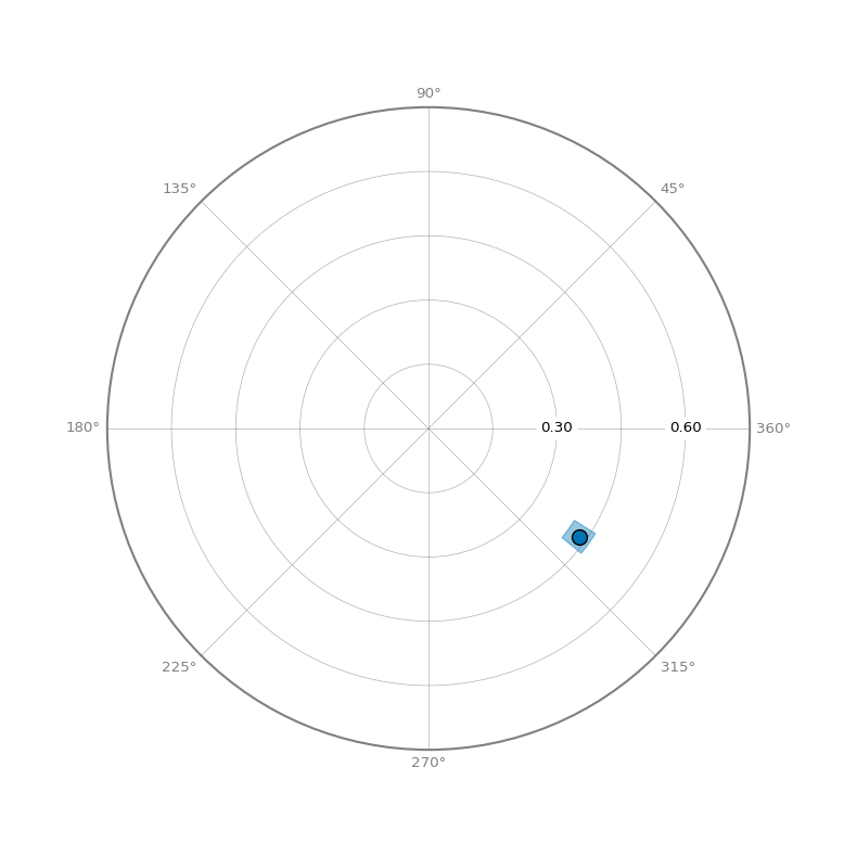
Circle Plot
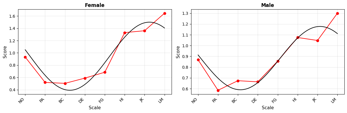
Curve Plot
4. Correlation-Based SSM Analysis
To examine how personality disorder symptoms relate to interpersonal problems, we can perform correlation-based SSM analysis by specifying external measures.
# Analyze narcissistic personality disorder symptoms
results_corr = ssm_analyze(
    data=jz2017,
    scales=scales,
    angles=angles,
    measures="NARPD",
)

results_corr.summary()
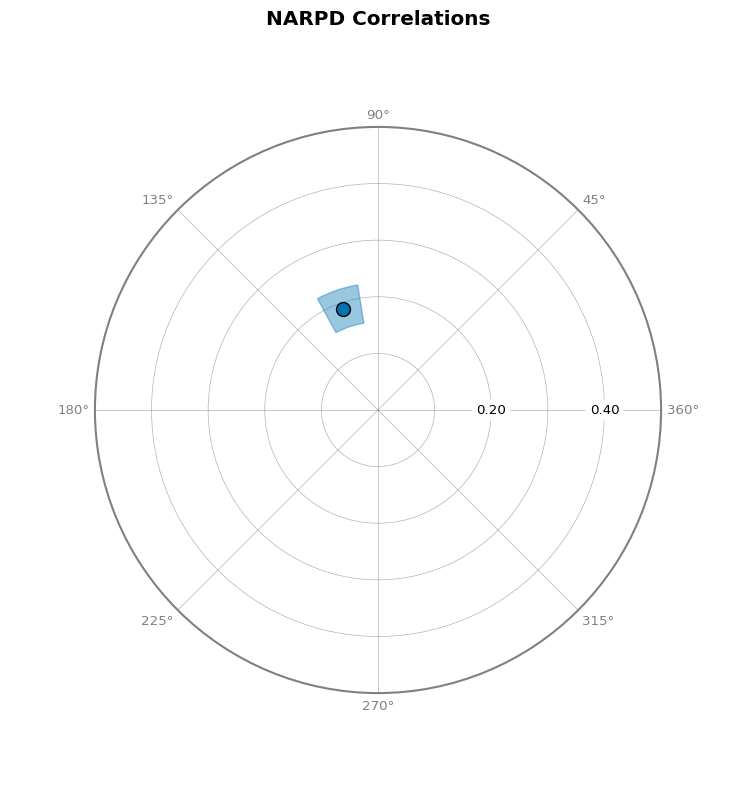
Statistical Basis:   Correlation Scores
Bootstrap Resamples: 2000
Confidence Level:    0.95
Listwise Deletion:   True
Scale Displacements: [90.0, 135.0, 180.0, 225.0, 270.0, 315.0, 360.0, 45.0]


                 Profile[NARPD]
┏━━━━━━━━━━━━━━┳━━━━━━━━━━┳━━━━━━━━━━┳━━━━━━━━━━┓
┃              ┃ Estimate ┃ Lower CI ┃ Upper CI ┃
┡━━━━━━━━━━━━━━╇━━━━━━━━━━╇━━━━━━━━━━╇━━━━━━━━━━┩
│ Elevation    │ 0.202    │ 0.167    │ 0.237    │
│ X-Value      │ -0.062   │ -0.094   │ -0.029   │
│ Y-Value      │ 0.179    │ 0.145    │ 0.212    │
│ Amplitude    │ 0.189    │ 0.155    │ 0.224    │
│ Displacement │ 108.967  │ 99.221   │ 118.54   │
│ Model Fit    │ 0.957    │          │          │
└──────────────┴──────────┴──────────┴──────────┘
5. Group Comparisons
Multiple Groups
# Analyze by gender
results_group = ssm_analyze(
    data=jz2017,
    scales=scales,
    angles=angles,
    grouping="Gender",
)

results_group.summary()
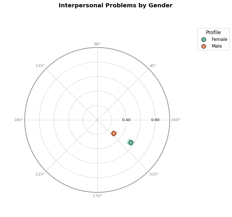
Statistical Basis:   Mean Scores
Bootstrap Resamples: 2000
Confidence Level:    0.95
Listwise Deletion:   True
Scale Displacements: [90.0, 135.0, 180.0, 225.0, 270.0, 315.0, 360.0, 45.0]


                 Profile[Female]
┏━━━━━━━━━━━━━━┳━━━━━━━━━━┳━━━━━━━━━━┳━━━━━━━━━━┓
┃              ┃ Estimate ┃ Lower CI ┃ Upper CI ┃
┡━━━━━━━━━━━━━━╇━━━━━━━━━━╇━━━━━━━━━━╇━━━━━━━━━━┩
│ Elevation    │ 0.946    │ 0.908    │ 0.984    │
│ X-Value      │ 0.459    │ 0.421    │ 0.497    │
│ Y-Value      │ -0.31    │ -0.356   │ -0.268   │
│ Amplitude    │ 0.554    │ 0.511    │ 0.599    │
│ Displacement │ 325.963  │ 321.939  │ 329.811  │
│ Model Fit    │ 0.889    │          │          │
└──────────────┴──────────┴──────────┴──────────┘
                  Profile[Male]
┏━━━━━━━━━━━━━━┳━━━━━━━━━━┳━━━━━━━━━━┳━━━━━━━━━━┓
┃              ┃ Estimate ┃ Lower CI ┃ Upper CI ┃
┡━━━━━━━━━━━━━━╇━━━━━━━━━━╇━━━━━━━━━━╇━━━━━━━━━━┩
│ Elevation    │ 0.884    │ 0.842    │ 0.926    │
│ X-Value      │ 0.227    │ 0.192    │ 0.261    │
│ Y-Value      │ -0.186   │ -0.225   │ -0.148   │
│ Amplitude    │ 0.294    │ 0.258    │ 0.33     │
│ Displacement │ 320.685  │ 313.649  │ 328.014  │
│ Model Fit    │ 0.824    │          │          │
└──────────────┴──────────┴──────────┴──────────┘
# Compare groups on circle plot
fig = results_group.plot_circle(colors="Set2", title="Interpersonal Problems by Gender")
Multiple Measures
# Compare multiple personality disorder symptoms
results_multi = ssm_analyze(
    data=jz2017,
    scales=scales,
    angles=angles,
    measures=["NARPD", "ASPD", "BORPD"],
)

results_multi.summary()
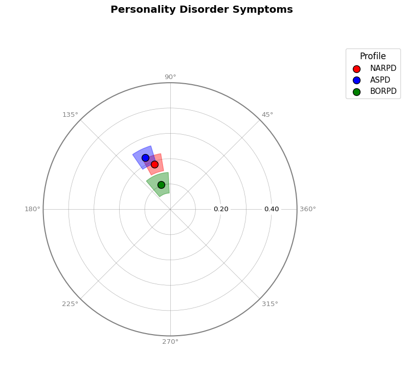
Statistical Basis:   Correlation Scores
Bootstrap Resamples: 2000
Confidence Level:    0.95
Listwise Deletion:   True
Scale Displacements: [90.0, 135.0, 180.0, 225.0, 270.0, 315.0, 360.0, 45.0]


                 Profile[NARPD]
┏━━━━━━━━━━━━━━┳━━━━━━━━━━┳━━━━━━━━━━┳━━━━━━━━━━┓
┃              ┃ Estimate ┃ Lower CI ┃ Upper CI ┃
┡━━━━━━━━━━━━━━╇━━━━━━━━━━╇━━━━━━━━━━╇━━━━━━━━━━┩
│ Elevation    │ 0.202    │ 0.168    │ 0.238    │
│ X-Value      │ -0.062   │ -0.094   │ -0.03    │
│ Y-Value      │ 0.179    │ 0.143    │ 0.211    │
│ Amplitude    │ 0.189    │ 0.154    │ 0.223    │
│ Displacement │ 108.967  │ 99.472   │ 118.732  │
│ Model Fit    │ 0.957    │          │          │
└──────────────┴──────────┴──────────┴──────────┘
                  Profile[ASPD]
┏━━━━━━━━━━━━━━┳━━━━━━━━━━┳━━━━━━━━━━┳━━━━━━━━━━┓
┃              ┃ Estimate ┃ Lower CI ┃ Upper CI ┃
┡━━━━━━━━━━━━━━╇━━━━━━━━━━╇━━━━━━━━━━╇━━━━━━━━━━┩
│ Elevation    │ 0.124    │ 0.089    │ 0.159    │
│ X-Value      │ -0.099   │ -0.133   │ -0.062   │
│ Y-Value      │ 0.203    │ 0.168    │ 0.237    │
│ Amplitude    │ 0.226    │ 0.191    │ 0.262    │
│ Displacement │ 115.927  │ 106.85   │ 124.367  │
│ Model Fit    │ 0.964    │          │          │
└──────────────┴──────────┴──────────┴──────────┘
                 Profile[BORPD]
┏━━━━━━━━━━━━━━┳━━━━━━━━━━┳━━━━━━━━━━┳━━━━━━━━━━┓
┃              ┃ Estimate ┃ Lower CI ┃ Upper CI ┃
┡━━━━━━━━━━━━━━╇━━━━━━━━━━╇━━━━━━━━━━╇━━━━━━━━━━┩
│ Elevation    │ 0.277    │ 0.243    │ 0.31     │
│ X-Value      │ -0.036   │ -0.069   │ -0.004   │
│ Y-Value      │ 0.097    │ 0.056    │ 0.138    │
│ Amplitude    │ 0.103    │ 0.064    │ 0.146    │
│ Displacement │ 110.358  │ 92.848   │ 130.012  │
│ Model Fit    │ 0.872    │          │          │
└──────────────┴──────────┴──────────┴──────────┘
# Visualize multiple measures
fig = results_multi.plot_circle(
    colors=["red", "blue", "green"], title="Personality Disorder Symptoms"
)
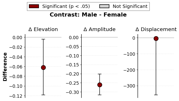
6. Contrast Analyses
Group Contrasts
To test whether groups differ significantly on SSM parameters, use
contrast=True:
# Contrast analysis between genders
results_contrast = ssm_analyze(
    data=jz2017,
    scales=scales,
    angles=angles,
    grouping="Gender",
    contrast=True,
)

results_contrast.summary()
Statistical Basis:   Mean Scores
Bootstrap Resamples: 2000
Confidence Level:    0.95
Listwise Deletion:   True
Scale Displacements: [90.0, 135.0, 180.0, 225.0, 270.0, 315.0, 360.0, 45.0]


                 Profile[Female]
┏━━━━━━━━━━━━━━┳━━━━━━━━━━┳━━━━━━━━━━┳━━━━━━━━━━┓
┃              ┃ Estimate ┃ Lower CI ┃ Upper CI ┃
┡━━━━━━━━━━━━━━╇━━━━━━━━━━╇━━━━━━━━━━╇━━━━━━━━━━┩
│ Elevation    │ 0.946    │ 0.906    │ 0.983    │
│ X-Value      │ 0.459    │ 0.422    │ 0.496    │
│ Y-Value      │ -0.31    │ -0.352   │ -0.267   │
│ Amplitude    │ 0.554    │ 0.512    │ 0.599    │
│ Displacement │ 325.963  │ 322.128  │ 329.684  │
│ Model Fit    │ 0.889    │          │          │
└──────────────┴──────────┴──────────┴──────────┘
                  Profile[Male]
┏━━━━━━━━━━━━━━┳━━━━━━━━━━┳━━━━━━━━━━┳━━━━━━━━━━┓
┃              ┃ Estimate ┃ Lower CI ┃ Upper CI ┃
┡━━━━━━━━━━━━━━╇━━━━━━━━━━╇━━━━━━━━━━╇━━━━━━━━━━┩
│ Elevation    │ 0.884    │ 0.842    │ 0.927    │
│ X-Value      │ 0.227    │ 0.191    │ 0.263    │
│ Y-Value      │ -0.186   │ -0.223   │ -0.147   │
│ Amplitude    │ 0.294    │ 0.258    │ 0.33     │
│ Displacement │ 320.685  │ 313.831  │ 327.899  │
│ Model Fit    │ 0.824    │          │          │
└──────────────┴──────────┴──────────┴──────────┘
             Profile[Male - Female]
┏━━━━━━━━━━━━━━┳━━━━━━━━━━┳━━━━━━━━━━┳━━━━━━━━━━┓
┃              ┃ Estimate ┃ Lower CI ┃ Upper CI ┃
┡━━━━━━━━━━━━━━╇━━━━━━━━━━╇━━━━━━━━━━╇━━━━━━━━━━┩
│ Elevation    │ -0.062   │ -0.118   │ -0.004   │
│ X-Value      │ -0.232   │ -0.282   │ -0.18    │
│ Y-Value      │ 0.124    │ 0.068    │ 0.18     │
│ Amplitude    │ -0.261   │ -0.317   │ -0.203   │
│ Displacement │ -5.278   │ 347.143  │ 2.851    │
│ Model Fit    │ -0.066   │          │          │
└──────────────┴──────────┴──────────┴──────────┘
# View contrast results (last row shows Male - Female differences)
GT(results_contrast.results.round(2))
| Label | Group | Measure | e_est | e_lci | e_uci | x_est | x_lci | x_uci | y_est | y_lci | y_uci | a_est | a_lci | a_uci | d_est | d_lci | d_uci | fit_est |
|---|---|---|---|---|---|---|---|---|---|---|---|---|---|---|---|---|---|---|
| Female | Female | 0.95 | 0.91 | 0.98 | 0.46 | 0.42 | 0.5 | -0.31 | -0.35 | -0.27 | 0.55 | 0.51 | 0.6 | 325.96 | 322.13 | 329.68 | 0.89 | |
| Male | Male | 0.88 | 0.84 | 0.93 | 0.23 | 0.19 | 0.26 | -0.19 | -0.22 | -0.15 | 0.29 | 0.26 | 0.33 | 320.68 | 313.83 | 327.9 | 0.82 | |
| Male - Female | Male - Female | -0.06 | -0.12 | -0.0 | -0.23 | -0.28 | -0.18 | 0.12 | 0.07 | 0.18 | -0.26 | -0.32 | -0.2 | -5.28 | 347.14 | 2.85 | -0.07 |
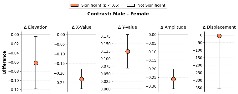
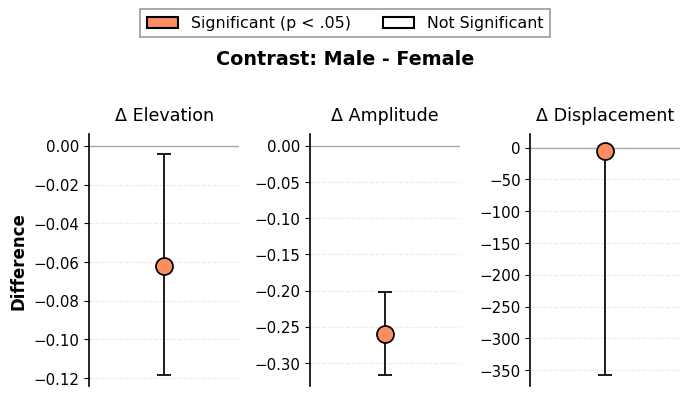
# Simplified contrast plot (drop X and Y parameters)
fig = results_contrast.plot_contrast(drop_xy=True)
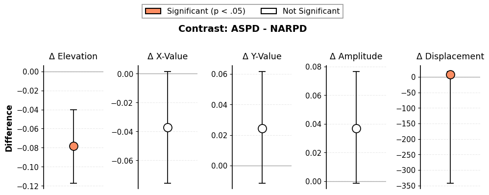
Measure Contrasts
# Compare two measures
results_meas_contrast = ssm_analyze(
    data=jz2017,
    scales=scales,
    angles=angles,
    measures=["NARPD", "ASPD"],
    contrast=True,
)

results_meas_contrast.summary()
Statistical Basis:   Correlation Scores
Bootstrap Resamples: 2000
Confidence Level:    0.95
Listwise Deletion:   True
Scale Displacements: [90.0, 135.0, 180.0, 225.0, 270.0, 315.0, 360.0, 45.0]


                 Profile[NARPD]
┏━━━━━━━━━━━━━━┳━━━━━━━━━━┳━━━━━━━━━━┳━━━━━━━━━━┓
┃              ┃ Estimate ┃ Lower CI ┃ Upper CI ┃
┡━━━━━━━━━━━━━━╇━━━━━━━━━━╇━━━━━━━━━━╇━━━━━━━━━━┩
│ Elevation    │ 0.202    │ 0.169    │ 0.235    │
│ X-Value      │ -0.062   │ -0.094   │ -0.028   │
│ Y-Value      │ 0.179    │ 0.146    │ 0.212    │
│ Amplitude    │ 0.189    │ 0.156    │ 0.224    │
│ Displacement │ 108.967  │ 99.04    │ 118.521  │
│ Model Fit    │ 0.957    │          │          │
└──────────────┴──────────┴──────────┴──────────┘
                  Profile[ASPD]
┏━━━━━━━━━━━━━━┳━━━━━━━━━━┳━━━━━━━━━━┳━━━━━━━━━━┓
┃              ┃ Estimate ┃ Lower CI ┃ Upper CI ┃
┡━━━━━━━━━━━━━━╇━━━━━━━━━━╇━━━━━━━━━━╇━━━━━━━━━━┩
│ Elevation    │ 0.124    │ 0.088    │ 0.16     │
│ X-Value      │ -0.099   │ -0.135   │ -0.063   │
│ Y-Value      │ 0.203    │ 0.169    │ 0.238    │
│ Amplitude    │ 0.226    │ 0.19     │ 0.262    │
│ Displacement │ 115.927  │ 107.14   │ 124.123  │
│ Model Fit    │ 0.964    │          │          │
└──────────────┴──────────┴──────────┴──────────┘
              Profile[ASPD - NARPD]
┏━━━━━━━━━━━━━━┳━━━━━━━━━━┳━━━━━━━━━━┳━━━━━━━━━━┓
┃              ┃ Estimate ┃ Lower CI ┃ Upper CI ┃
┡━━━━━━━━━━━━━━╇━━━━━━━━━━╇━━━━━━━━━━╇━━━━━━━━━━┩
│ Elevation    │ -0.079   │ -0.117   │ -0.04    │
│ X-Value      │ -0.037   │ -0.076   │ 0.001    │
│ Y-Value      │ 0.024    │ -0.012   │ 0.062    │
│ Amplitude    │ 0.037    │ -0.001   │ 0.077    │
│ Displacement │ 6.96     │ 356.639  │ 17.454   │
│ Model Fit    │ 0.007    │          │          │
└──────────────┴──────────┴──────────┴──────────┘
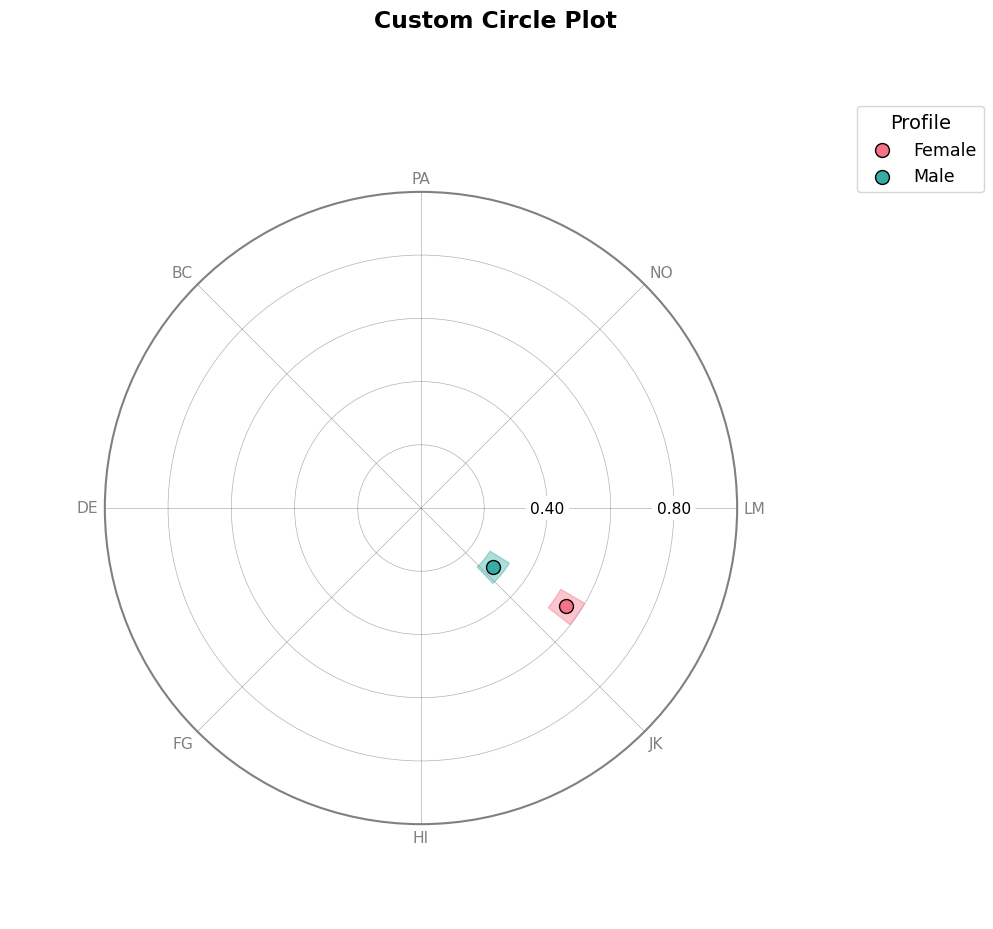
7. Customizing Visualizations
All plot functions support extensive customization:
# Circle plot with custom options
fig = results_group.plot_circle(
    colors="husl",  # Color palette
    fontsize=14,  # Font size
    figsize=(10, 10),  # Figure size
    title="Custom Circle Plot",
    angle_labels=scales,  # Custom angle labels
)
# Curve plot with custom options
fig = results_group.plot_curve(
    angle_labels=scales,
    base_size=12,
    figsize=(12, 5),
)

# Contrast plot with custom colors
fig = results_contrast.plot_contrast(
    sig_color="darkred",
    ns_color="lightgray",
    fontsize=14,
    drop_xy=True,
)
8. Saving Plots
All plots return matplotlib Figure objects that can be saved:
# Save plots
fig1 = results.plot_circle()
fig1.savefig("circle_plot.png", dpi=300, bbox_inches="tight")

fig2 = results.plot_curve()
fig2.savefig("curve_plot.png", dpi=300, bbox_inches="tight")

Summary
The circumplex package provides a comprehensive toolkit for SSM analysis:
ssm_analyze(): Performs mean-based or correlation-based SSM analysisplot_circle(): Visualizes amplitude/displacement on circular plotsplot_curve(): Shows fitted curves with observed dataplot_contrast(): Displays parameter differences between groups
All functions support: - Single or multiple groups - Single or multiple measures - Bootstrap confidence intervals - Contrast analyses - Extensive customization options